About Machine Learning ( Part 2: Linear Regression )

Dataset

In prediction tasks, we often use independent features to predict a dependent variable. If we have a dataset:

$$
{ x_d^{(i)}, t^{(i)} }
$$

where:

• $x_d^{(i)}$: The $d$-th feature of the $i$-th instance in the dataset.
• $t^{(i)}$: The target value (dependent variable) for the $i$-th instance.
• $i = 1, \dots, N$: $i$ indexes the instances, and $N$ is the total number of instances in the dataset. ( Here $i$ is not power )
• $d = 1, \dots, D$: $d$ indexes the features, and $D$ is the total number of independent features.

Each feature in the dataset can be expressed as:

$$
x_d^{(i)}
$$

For simplicity, the following focuses on a single feature $x$, meaning $D = 1$.

Polynomial

This is a curve fitting problem, where we aim to fit a polynomial function to model the relationship between the independent variable $x$ and the dependent variable $t$.

A polynomial model is expressed as:

$$
h(x, \omega) = \omega_0 + \omega_1 x + \omega_2 x^2 + \cdots + \omega_M x^M
$$

• $h(x, \omega)$: The predicted output (dependent variable) for a given input $x$.
• $\omega_0, \omega_1, \dots, \omega_M$: The coefficients (parameters) of the polynomial.
• $M$: The order of the polynomial, which represents the highest power of $x$ used in the model.

This expanded form explicitly shows all terms of the polynomial up to order $M$.

It can also be written in a more compact form using summation:

$$
h(x, \omega) = \omega_0 + \sum_{j=1}^{M} \omega_j x^j
$$

Here:

• The summation $\sum_{j=1}^{M} \omega_j x^j$ compactly represents all terms from $j = 1$ (first-order) to $j = M$ (highest-order).
• $\omega_0$: The constant term (bias), which is excluded from the summation since it is independent of $x$.

Linear Regression

For a straight line, the model is a linear function of the form:

$$
f(x, \omega) = \omega_0 + \omega_1 x
$$

Where:

• $M = 1$, indicating that the polynomial is of degree 1 (a straight line).
• $f(x, \omega) = \omega_0 + \omega_1 x$ is the equation of the line.
• $\omega_1$ represents the slope of the line, and $\omega_0$ represents the y-intercept in the equation.

We can use optimization to minimize the overall error. The cost function $J(\omega)$ is defined as:

$$
J(\omega) = \frac{1}{2} \sum_{n=1}^{N} \left(t_n - f(x_n, \omega)\right)^2
$$

Where:

• $J(\omega)$ is the cost function that we aim to minimize ( MSE ).
• $t_n$ is the target value (actual value) for the $n$-th data point.
• $f(x_n, \omega)$ is the predicted value from the model for the $n$-th data point.
• $N$ is the total number of data points in the dataset.

Gradient Descent

Gradient Descent is an optimization algorithm used to minimize the cost function. The idea is to adjust the parameters ($\omega_0$, $\omega_1$, etc.) in the direction of the negative gradient of the cost function to reduce the error. The general update rule is:

$$
\omega \leftarrow \omega - \lambda \nabla J(\omega)
$$

Here:

• $\omega$ represents the model parameters (e.g., $\omega_0, \omega_1$).
• $\lambda$ is the learning rate, controlling the step size in each update.
• $\nabla J(\omega)$ is the gradient of the cost function with respect to $\omega$.

---

The cost function for linear regression is:

$$
J(\omega) = \frac{1}{2} \sum_{n=1}^N \left( (\omega_0 + \omega_1 x_n) - t_n \right)^2
$$

We compute the partial derivatives of $J(\omega)$ with respect to each parameter:

1. Gradient with respect to $\omega_0$:

   $$
   \frac{\partial J(\omega)}{\partial \omega_0} = \sum_{n=1}^N \left( (\omega_0 + \omega_1 x_n) - t_n \right)
   $$

2. Gradient with respect to $\omega_1$:
   $$
   \frac{\partial J(\omega)}{\partial \omega_1} = \sum_{n=1}^N \left( (\omega_0 + \omega_1 x_n) - t_n \right) x_n
   $$

---

Using the gradients, the parameters are updated as follows:

1. For $\omega_0$:

   $$
   \omega_0 \leftarrow \omega_0 - \lambda \sum_{n=1}^N \left( (\omega_0 + \omega_1 x_n) - t_n \right)
   $$

2. For $\omega_1$:
   $$
   \omega_1 \leftarrow \omega_1 - \lambda \sum_{n=1}^N \left( (\omega_0 + \omega_1 x_n) - t_n \right) x_n
   $$

---

1. Initialize $\omega_0$ and $\omega_1$ with some random values (e.g., $0$).
2. Compute the gradients $\frac{\partial J(\omega)}{\partial \omega_0}$ and $\frac{\partial J(\omega)}{\partial \omega_1}$.
3. Update $\omega_0$ and $\omega_1$ using the update rules.
4. Repeat the process until:
   • The cost function $J(\omega)$ converges to a minimum, or
   • The number of iterations reaches a predefined limit.

Demo Code

Linear Regression with Multiple Features

The model can be written as:

$$
\hat{y} = \theta_0 + \theta_1 x_1 + \theta_2 x_2 + \dots + \theta_D x_D
$$

Where:

• $D$ is the number of attributes (features) in the dataset.
• $x_1, x_2, \dots, x_D$ are the features of the data.
• $\theta_0$ is the intercept (bias term).
• $\theta_1, \theta_2, \dots, \theta_D$ are the weights (coefficients) corresponding to each feature.

This equation can also be expressed in matrix form for computational efficiency.

---

In matrix form, the prediction $\hat{y}$ is expressed as:

$$
\hat{y} = X \theta
$$

Where:

• $X$ is the design matrix of size $N \times (D+1)$, where:
  • $N$ is the number of instances (data points).
  • The first column of $X$ is all ones, representing the bias term ($\theta_0$).
  • The remaining columns correspond to the feature values.

For example, $X$ can look like this:

$$
X =
\begin{bmatrix}
1 & x_1^{(1)} & x_2^{(1)} & \dots & x_D^{(1)} \newline
1 & x_1^{(2)} & x_2^{(2)} & \dots & x_D^{(2)} \newline
\vdots & \vdots & \vdots & \ddots & \vdots \newline
1 & x_1^{(N)} & x_2^{(N)} & \dots & x_D^{(N)}
\end{bmatrix}
$$

• $\theta$ is the vector of coefficients:
  $$
  \theta =
  \begin{bmatrix}
  \theta_0 \newline
  \theta_1 \newline
  \theta_2 \newline
  \vdots \newline
  \theta_D
  \end{bmatrix}
  $$

---

To find the optimal values of $\theta$, we minimize the cost function, which is typically the Mean Squared Error (MSE):

$$
J(\theta) = \frac{1}{2N} \sum_{i=1}^N \left( \hat{y}^{(i)} - t^{(i)} \right)^2
$$

In matrix form, this is written as:

$$
J(\theta) = \frac{1}{2N} | X \theta - t |^2
$$

Where $t$ is the vector of true target values:

$$
t =
\begin{bmatrix}
t^{(1)} \newline
t^{(2)} \newline
\vdots \newline
t^{(N)}
\end{bmatrix}
$$

---

By setting the gradient of $J(\theta)$ with respect to $\theta$ to zero, we derive the closed-form solution:
$$
\hat{\theta} = (X^T X)^{-1} X^T t
$$

Where:

• $X^T$ is the transpose of the design matrix.
• $(X^T X)^{-1}$ is the inverse of the matrix product $X^T X$.

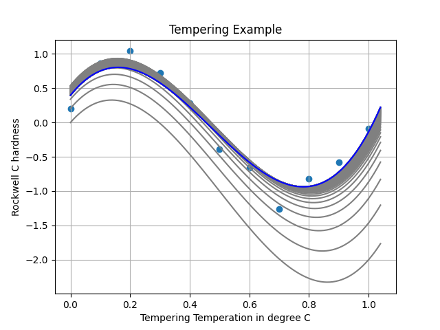
Higher Order Polynomials

In polynomial regression, we model the relationship between the input variable $x$ and output $f(x, \omega)$ using a higher degree polynomial:

$$
f(x, \omega) = \omega_0 + \omega_1 x + \omega_2 x^2 + \dots + \omega_M x^M = \sum_{j=0}^{M} \omega_j x^j
$$

• $x$ is the input feature, and $\omega_j$ are the coefficients.
• $M$ is the degree of the polynomial, which determines the complexity of the model.

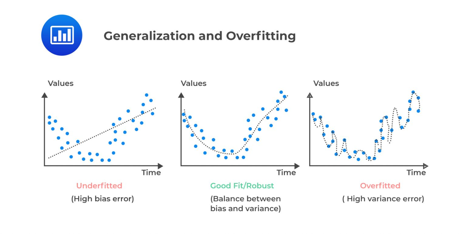
Choosing $M$ (Degree of Polynomial):

• Small $M$: Captures simple relationships; less prone to overfitting.
• Large $M$: Can overfit the data by capturing noise.
• Selection: Cross-validation is used to determine the best $M$ to balance fit and generalization.

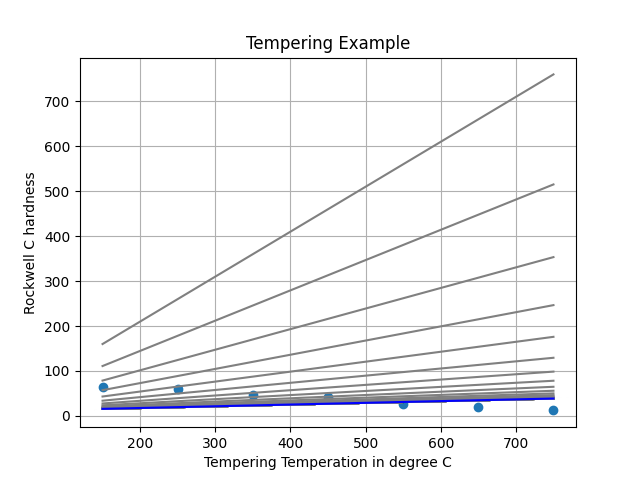
Overfitting & Regularization

In linear regression, overfitting occurs when the model becomes too complex and starts to fit noise in the training data. To prevent overfitting, we use regularization to penalize large coefficients and simplify the model.

The regularized cost function is:

$$
E(\omega) = \frac{1}{2} \sum_{n=1}^{N} (f(x_n, \omega) - t_n)^2 + \frac{\lambda}{2} |\omega|^2
$$

Where:

• $f(x_n, \omega)$ is the model’s prediction for the $n$-th data point.
• $t_n$ is the true target for the $n$-th data point.
• $\lambda$ is the regularization parameter that controls the strength of the penalty.
• $|\omega|^2$ is the squared L2 norm of the weights, i.e., the sum of the squares of the coefficients.

The $\lambda$ parameter allows you to control the trade-off between fitting the data well and keeping the model simple.