About Machine Learning ( Part 3: Logistic Regression )

Classification Problem

In machine learning, when we are predicting a discrete label, such as determining whether an email is spam or not, we are dealing with a classification problem. Logistic regression is commonly used for binary classification tasks, where the goal is to predict one of two classes, typically represented as 0 or 1.

The logistic function (also called the sigmoid function) is the core of logistic regression, as it maps input features to probabilities between 0 and 1. These probabilities represent the likelihood of the sample belonging to a particular class.

The logistic function is defined as:

$$
\sigma(z) = \frac{1}{1 + e^{-z}}
$$

Where $z = \omega_0 + \mathbf{\omega}^T \mathbf{x}$, the linear combination of the input features $\mathbf{x}$ and the model’s parameters $\mathbf{\omega}$.

Model Representation

In logistic regression, we aim to predict the probability that an observation $\mathbf{x}$ belongs to class 1. The predicted probability is given by the following equation:

$$
p(C = 1|\mathbf{x}) = \sigma(\omega_0 + \mathbf{\omega}^T \mathbf{x}) = \frac{1}{1 + e^{-(\omega_0 + \mathbf{\omega}^T \mathbf{x})}}
$$

where:

• $p(C = 1|\mathbf{x})$: The probability that the class label $C$ is 1, given the input features $\mathbf{x}$.
• $\omega_0$: The bias term, which helps adjust the output independently of the input features.
• $\mathbf{\omega}$: The weight vector that contains the coefficients for each feature.
• $\mathbf{\omega}^T \mathbf{x}$: The dot product between the weight vector $\mathbf{\omega}$ and the feature vector $\mathbf{x}$, representing the weighted sum of the input features.

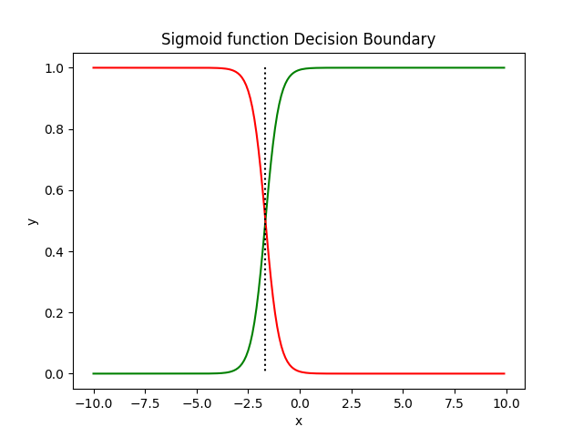
Decision Boundary

In binary classification, the decision boundary is the point where the model predicts equal probabilities for both classes, meaning the probability of being in class 0 is 0.5 and the probability of being in class 1 is also 0.5. This boundary helps separate the two classes.

We calculate this boundary by setting the predicted probability equal to 0.5:

$$
p(C = 1|\mathbf{x}) = 0.5
$$

This happens when the output of the logistic function equals 0.5. Solving for the decision boundary, we get:

$$
\sigma(\omega_0 + \mathbf{\omega}^T \mathbf{x}) = 0.5
$$

This implies:

$$
\omega_0 + \mathbf{\omega}^T \mathbf{x} = 0
$$

This equation represents the decision boundary where the model will predict a 50% chance of the sample belonging to either class. Points on this boundary are classified as uncertain.

Maximum Likelihood Estimation (MLE)

In logistic regression, the goal is to find the parameters $\mathbf{\omega} = (\omega_0, \omega_1, …, \omega_d)$ that maximize the likelihood of observing the training data. The likelihood function $L(\mathbf{\omega})$ is the probability of the observed labels given the feature vectors.

If We assume that the data is independent and
identically distributed (IDD). The likelihood function will be:

$$
L(\mathbf{\omega}) = \prod_{i=1}^{N} p(t_i | \mathbf{x}_i; \mathbf{\omega})
$$

Where:

• $N$: The number of training samples.
• $t_i$: The actual label for the $i$-th sample.
• $\mathbf{x}_i$: The feature vector for the $i$-th sample.
• $p(t_i | \mathbf{x}_i; \mathbf{\omega})$: The probability of observing label $t_i$ given the features $\mathbf{x}_i$ and parameters $\mathbf{\omega}$.

Maximizing this likelihood function helps us find the optimal values for the model’s parameters.

Log-Likelihood Function

However, when we have many samples ($N$ is large) and each probability $p(t_i | \mathbf{x}_i; \mathbf{\omega})$ is a value less than 1, the product of these probabilities becomes very small. This leads to a problem called Numerical Underflow, where the computer cannot handle such small numbers.

So, maximizing the likelihood function directly is difficult due to the product of probabilities. Instead, we take the log-likelihood, which simplifies the optimization by turning the product into a sum:

$$
\ln(L(\mathbf{\omega})) = \sum_{i=1}^{N} \left[ t_i \ln(p(t_i = 1|\mathbf{x}_i; \mathbf{\omega})) + (1 - t_i) \ln(1 - p(t_i = 1|\mathbf{x}_i; \mathbf{\omega})) \right]
$$

This form assumes a binary classification scenario, where each label $t_i$ can only be either 0 or 1. In such a case:

• If $t_i = 1$, we calculate the log of the predicted probability for class 1: $\ln(p(t_i = 1|\mathbf{x}_i; \mathbf{\omega}))$.
• If $t_i = 0$, we calculate the log of the probability of class 0, which is $1 - p(t_i = 1|\mathbf{x}_i; \mathbf{\omega})$: $\ln(1 - p(t_i = 1|\mathbf{x}_i; \mathbf{\omega}))$.

This reflects the basic assumption of binary classification in logistic regression, where the goal is to predict the probability of an input sample belonging to class 1 (or class 0, which is just the complement of class 1).

Gradient Descent for Optimization

We use gradient descent to maximize the log-likelihood function. Gradient descent involves computing the gradient of the log-likelihood with respect to the parameters $\mathbf{\omega}$, and then updating the parameters in the direction that increases the log-likelihood.

The gradient of the log-likelihood function with respect to each parameter $\omega_d$ is:

$$ \frac{\partial \ln(L(\mathbf{\omega}))}{\partial \omega_d} = \sum_{i=1}^{N} ( t_i - p(C = 1 \mid \mathbf{x}_i; \mathbf{\omega})) x_{i,d} $$

Where:

• $x_{i,d}$ is the $d$-th feature of the $i$-th sample.
• $p(C = 1|\mathbf{x}_i; \mathbf{\omega})$ is the predicted probability of class 1 for the $i$-th sample.
• $t_i$ is the true label of the $i$-th sample, where $t_i = 1$ if the sample belongs to class 1 (positive class), and $t_i = 0$ if it belongs to class 0 (negative class).

Explanation:

• The term $(t_i - p(C = 1|\mathbf{x}_i; \mathbf{\omega}))$ represents the error between the true label and the predicted probability for the $i$-th sample.
• The product of this error and the corresponding feature $x_{i,d}$ allows us to adjust the weight $\omega_d$ based on how the feature $x_{i,d}$ contributes to the error.

By summing over all $N$ samples, the gradient is computed for each parameter $\omega_d$. Using the gradient, we update the parameters $\mathbf{\omega}$ using the following rule:

$$
\omega_d \leftarrow \omega_d - \lambda \frac{\partial \ln(L(\mathbf{\omega}))}{\partial \omega_d}
$$

Where:

• $\lambda$ is the learning rate, which controls the step size during optimization.

Demo Code

Confusion Matrix

The confusion matrix is a table that summarizes the performance of a classifier on a set of test data for which the true values are known.

	Predicted Positive	Predicted Negative
Actual Positive	True Positive (TP)	False Negative (FN)
Actual Negative	False Positive (FP)	True Negative (TN)

• True Positive (TP): Correctly predicted positive instances.
• True Negative (TN): Correctly predicted negative instances.
• False Positive (FP): Negative instances incorrectly predicted as positive.
• False Negative (FN): Positive instances incorrectly predicted as negative.

Accuracy

Accuracy measures the proportion of correctly classified instances (both positive and negative) out of all predictions.

Formula:

$$
\text{Accuracy} = \frac{\text{TP} + \text{TN}}{\text{TP} + \text{TN} + \text{FP} + \text{FN}}
$$

When to use Accuracy:

• When the dataset is balanced, meaning the number of positive and negative instances is roughly equal.

---

Precision (Positive Predictive Value)

Precision quantifies the proportion of positive predictions that are correct.

Formula:

$$
\text{Precision} = \frac{\text{TP}}{\text{TP} + \text{FP}}
$$

Use case for Precision:

• When false positives have a high cost (e.g., flagging legitimate emails as spam).

---

Recall (Sensitivity or True Positive Rate)

Recall measures the proportion of actual positives that are correctly identified.

Formula:

$$
\text{Recall} = \frac{\text{TP}}{\text{TP} + \text{FN}}
$$

Use case for Recall:

• When false negatives have a high cost (e.g., failing to detect a disease in medical testing).

---

F1-Score (Harmonic Mean of Precision and Recall)

The F1-Score combines Precision and Recall into a single metric, especially useful when you need to balance the trade-off between the two.

Formula:

$$
F_1 = 2 \cdot \frac{\text{Precision} \cdot \text{Recall}}{\text{Precision} + \text{Recall}}
$$

Why use F1-Score?

• It is beneficial when dealing with imbalanced datasets, as it considers both false positives and false negatives.

---

Key Insights

• Accuracy works well on balanced datasets but may be misleading when classes are imbalanced.
• Precision is crucial when false positives are costly.
• Recall is critical when false negatives are costly.
• F1-Score provides a balanced measure when both Precision and Recall are important.

By carefully analyzing the confusion matrix and the derived metrics, you can fine-tune your model for optimal performance, depending on the specific requirements of your application.