About Machine Learning ( Part 7: Artificial Neural Network )

Bayes’ theorem

$$
P(y|X) = \frac{P(X|y) P(y)}{P(X)}
$$

where:

• $P(y|X)$: Posterior probability of class $y$ given input $X$.
• $P(X|y)$: Likelihood of seeing $X$ if the class is $y$.
• $P(y)$: Prior probability of class $y$.
• $P(X)$: Total probability of $X$ (normalization factor).

Bayes Network (Bayesian Network, BN)

A Bayesian network (BN) is a graphical model representing probabilistic dependencies between variables. It consists of:

• Nodes: Represent variables (e.g., symptoms, diseases).
• Edges: Represent conditional dependencies.

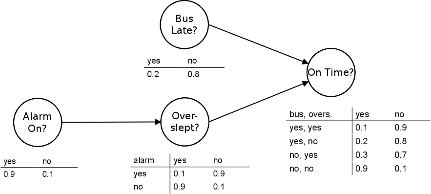
Bayesian Inference in BN

Using Bayes’ rule, we can infer probabilities, such as:

$$
P(F|T, C) = \frac{P(T, C | F) P(F)}{P(T, C)}
$$

Bayesian networks are widely used in medical diagnosis, fraud detection, and AI decision-making.

Artificial Neural Network (ANN)

The Perceptron

A perceptron is a simple artificial neuron that performs binary classification. It computes a weighted sum of inputs and applies an activation function:

$$
y = \begin{cases}
1, & \text{if } w \cdot X + b > 0 \newline
0, & \text{otherwise}
\end{cases}
$$

where:

• $X$ is the input vector.
• $w$ is the weight vector.
• $b$ is the bias term.

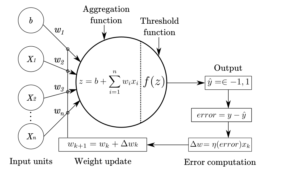
Learning in Perceptrons

The perceptron updates its weights using a simple rule:

$$
w \leftarrow w + \Delta w
$$

where:

$$
\Delta w = \eta (y_{\text{true}} - y_{\text{pred}}) X
$$

• $\eta$ is the learning rate.
• The perceptron adjusts weights only when it makes an error.

Limitations of the Perceptron:

• Can only solve linearly separable problems (e.g., AND, OR gates).
• Fails for XOR problems, motivating more advanced learning rules.
• So activation funtion are usually used.

Delta Rule

The Delta Rule is a gradient descent learning rule used in single-layer perceptrons and neural networks to minimize error and update weights. The main idea behind this rule is to adjust the weights based on the gradient of the error to minimize the loss function (often the Mean Squared Error, MSE). The Delta Rule is a specific case of the Gradient Descent method.

Assume the output of a perceptron is calculated by the following formula:

$$
y = f(w_1 x_1 + w_2 x_2 + \dots + w_n x_n + b)
$$

Where:

• $x_i$ is the input value,
• $w_i$ is the corresponding weight,
• $b$ is the bias,
• $f(\cdot)$ is the activation function (usually a linear or Sigmoid function),
• $y$ is the output,
• $t$ is the target label (the true value),
• $e = t - y$ is the error (difference between predicted and true output).

The Delta Rule updates the weights as follows:

$$
\Delta w_i = \eta (t - y) x_i
$$

Where:

• $\eta$ is the learning rate that controls the step size of the updates,
• $(t - y)$ is the error,
• $x_i$ is the input used to adjust the corresponding weight.

The weight update rule becomes:

$$
w_i \leftarrow w_i + \Delta w_i
$$

Derivation of the Delta Rule

The Error Function (Mean Squared Error)

To understand how the Delta Rule works, we first need to define the error function. The Mean Squared Error (MSE) is commonly used as the error metric in neural networks, especially for regression tasks. It measures the difference between the target output $t$ and the predicted output $y$:

$$
E = \frac{1}{2} (t - y)^2
$$

Where:

• $t$ is the target value (the true label),
• $y$ is the predicted output from the neural network.

The reason we use a factor of $\frac{1}{2}$ is to simplify the derivative when we apply the chain rule during weight updates.

The Goal: Weight Update

The goal of the Delta Rule is to update the weights so that the error $E$ is minimized. We do this by adjusting the weights in the direction that reduces the error. To achieve this, we compute the gradient (partial derivative) of the error function with respect to the weights $w_i$.

The output $y$ of a single output unit in the network is determined by:

$$
y = f(net)
$$

Where:

• $net = \sum_{i} w_i x_i + b$ is the weighted sum of inputs,
• $f(\cdot)$ is the activation function applied to the weighted sum (in this case, we’ll focus on the Sigmoid function).

To update the weights, we need the partial derivative of the error $E$ with respect to each weight $w_i$. This is done using the chain rule:

$$
\frac{\partial E}{\partial w_i} = \frac{\partial E}{\partial y} \cdot \frac{\partial y}{\partial w_i}
$$

Compute $\frac{\partial E}{\partial y}$

The first term we need is the derivative of the error with respect to the output $y$. Since $E$ is the squared error, we can differentiate:

$$
\frac{\partial E}{\partial y} = -(t - y)
$$

This represents how much the error changes with respect to the output $y$.

Compute $\frac{\partial y}{\partial w_i}$

Next, we calculate the derivative of the output $y$ with respect to each weight $w_i$. The output $y$ is the result of applying the activation function $f$ to the weighted sum $net$:

$$
y = f(net)
$$

Using the chain rule, we get:

$$
\frac{\partial y}{\partial w_i} = \frac{\partial f(net)}{\partial net} \cdot \frac{\partial net}{\partial w_i}
$$

Where:

• $\frac{\partial f(net)}{\partial net} = f’(net)$ is the derivative of the activation function with respect to the net input,
• $\frac{\partial net}{\partial w_i} = x_i$, since $net = \sum w_i x_i + b$.

Thus:

$$
\frac{\partial y}{\partial w_i} = f’(net) \cdot x_i
$$

Combine Terms for the Gradient

Now, we combine the terms to compute the gradient of the error with respect to the weight $w_i$:

$$
\frac{\partial E}{\partial w_i} = -(t - y) \cdot f’(net) \cdot x_i
$$

This expression tells us how much to adjust each weight $w_i$ to minimize the error.

Derivative of the Sigmoid Activation Function

For the Sigmoid activation function, the output $o$ is given by:

$$
o = f(net) = \frac{1}{1 + e^{-net}}
$$

The derivative of the Sigmoid function with respect to the net input $net$ is:

$$
f’(net) = o(1 - o)
$$

Where $o$ is the output of the Sigmoid function.

The Final Weight Update Rule

We can now substitute the derivative of the Sigmoid function into the weight update formula. The Delta Rule for updating weights is:

$$
\Delta w_i = \eta (t - y) \cdot o \cdot (1 - o) \cdot x_i
$$

Where:

• $\eta$ is the learning rate, which controls how much the weights are adjusted at each step,
• $(t - y)$ is the error between the target and predicted output,
• $o(1 - o)$ is the derivative of the Sigmoid activation function,
• $x_i$ is the input corresponding to the weight $w_i$.

Finally, the weights are updated as follows:

$$
w_i \leftarrow w_i + \Delta w_i
$$

This update ensures that the weights move in the direction that minimizes the error.

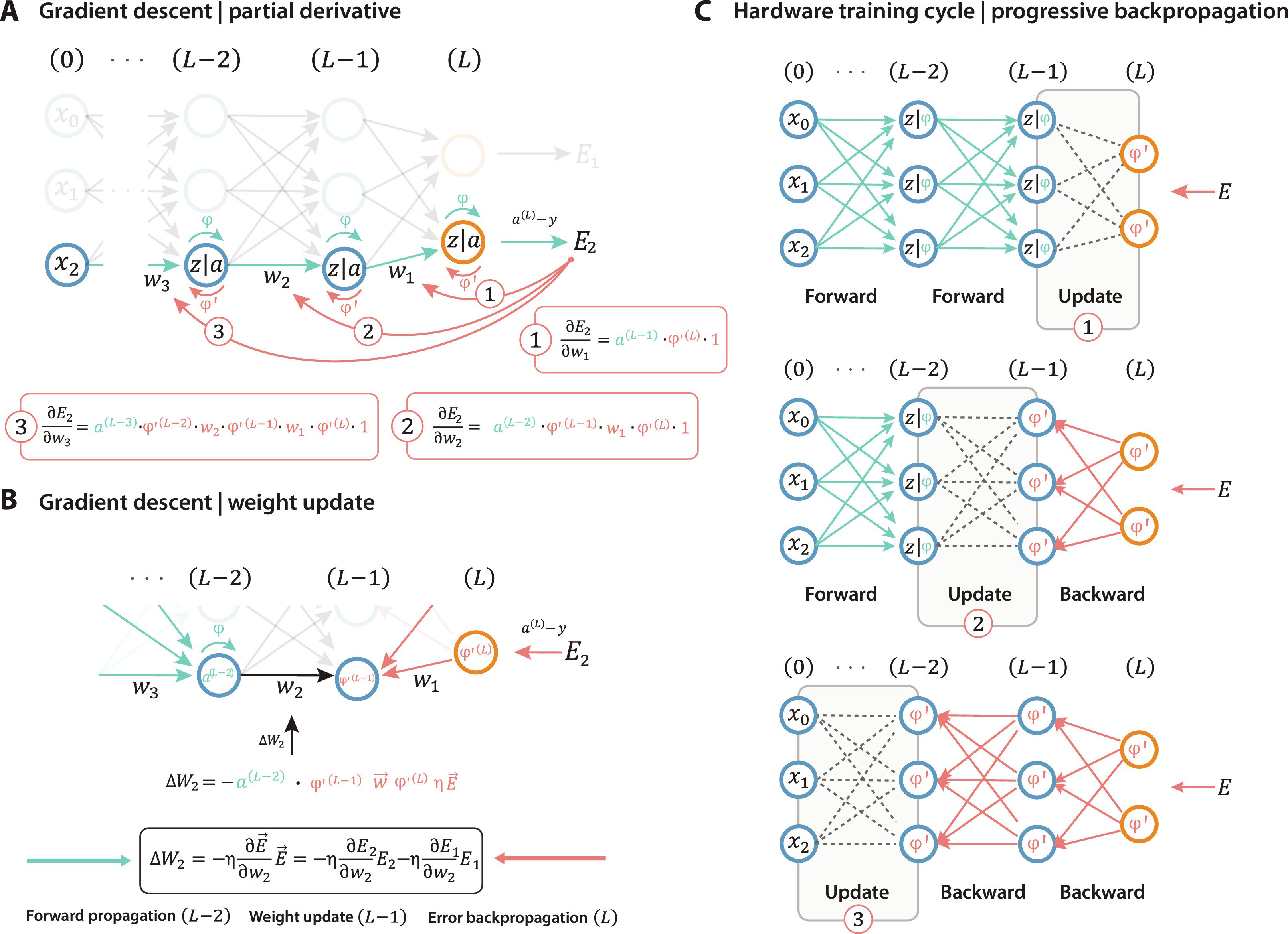
The Difference in the Calculation of $\delta_k$ for Output and Hidden Layers

The calculation of the error signal $\delta_k$ is different in the output layer and the hidden layer because:

• Output layer error is directly related to the target error, and we can compute the gradient directly.
• Hidden layer error is not directly related to the target, so we need to propagate the error backwards from downstream layers (closer to the output layer).

Output Layer’s $\delta_k$: Direct Calculation from Error

In the output layer, the error can be directly calculated because the output neurons compare their output values $o_k$ directly with the target values $y_k$. Thus, the error signal $\delta_k$ is calculated directly based on the loss function.

For the Mean Squared Error (MSE) loss function:

$$
E = \frac{1}{2} \sum_k (y_k - o_k)^2
$$

We take the partial derivative with respect to $net_k$:

$$
\delta_k = \frac{\partial E}{\partial net_k} = \frac{\partial E}{\partial o_k} \cdot \frac{\partial o_k}{\partial net_k}
$$

Where:

• $\frac{\partial E}{\partial o_k} = -(y_k - o_k)$ (the error term),
• $\frac{\partial o_k}{\partial net_k}$ depends on the activation function (e.g., Sigmoid: $o_k(1 - o_k)$).

Thus, for the Sigmoid activation function:

$$
\delta_k = -(y_k - o_k) \cdot o_k (1 - o_k)
$$

This calculation is specific to the output layer because the error term $y_k - o_k$ is directly available.

Hidden Layer’s $\delta_h$: Backpropagating Error from Downstream

In the hidden layer, the error cannot be directly calculated because the hidden neurons do not directly compare their outputs with target values. So, how do we know how much a hidden neuron contributes to the final error?

The answer is: The error signal propagates backward from downstream layers!

What are downstream layers?

• Neural networks perform forward propagation for computing outputs, but the error is propagated backward.
• Hidden neurons influence multiple output neurons, so their error needs to be propagated back from those output neurons.
• “Downstream” refers to layers closer to the output layer, and “upstream” refers to layers closer to the input layer.

Calculating the Hidden Layer’s Error Signal $\delta_h$

For a hidden layer neuron $h$, there is no direct error, so its gradient comes from downstream layers (the output layer or deeper hidden layers).

Using the Chain Rule, we calculate:

$$
\delta_h = \sum_k \left( \delta_k \cdot \omega_{kh} \right) \cdot o_h (1 - o_h)
$$

Where:

• $\delta_k$ is the downstream (output layer) error signal,
• $\omega_{kh}$ is the weight from the hidden layer neuron $h$ to the output layer neuron $k$,
• $o_h(1 - o_h)$ is the derivative of the activation function for the hidden layer neuron.
• $\sum_k (\delta_k \cdot \omega_{kh})$: If the hidden layer neuron $h$ is connected to multiple output neurons $k$, its error is the weighted sum of all these error signals.

Backpropagation

Backpropagation is the core algorithm behind training multi-layer neural networks. It efficiently computes the gradient of the loss function with respect to the network’s weights, enabling the network to learn from data through gradient descent.

Backpropagation Algorithm

Step 1: Initialize the network

• Create a feed-forward network with:
  • $n_{in}$ input neurons
  • $n_h$ hidden neurons
  • $n_{out}$ output neurons
• Assign random small weights (e.g., between $-0.05$ and $0.05$) to break symmetry.

Step 2: Forward Propagation
For each training example $\mathbf{x}$:

1. Compute the weighted sum of inputs for each neuron.
2. Apply an activation function (e.g., Sigmoid) to get the output.

Step 3: Compute Errors

1. Compute the error at the output layer:
   $$
   \delta_j = \sigma_j (1 - \sigma_j) (t_j - out_j)
   $$
   where:

   • $\sigma_j$ is the output of the neuron
   • $t_j$ is the target value
   • $out_j$ is the actual output

2. Compute the error at the hidden layers by propagating errors backward:
   $$
   \delta_j = \sigma_j (1 - \sigma_j) \sum_{k \in \text{downstream}} w_{kj} \delta_k
   $$

Step 4: Update Weights
Each weight $w_{ij}$ is updated using gradient descent:
$$
w_{ij} \leftarrow w_{ij} + \eta \delta_j x_i
$$
where $\eta$ is the learning rate.

Numerical Example of Backpropagation

Let’s go through an example using a small network.

Network Structure

• Input layer: 2 neurons ($x_1, x_2$)
• Hidden layer: 2 neurons ($h_1, h_2$)
• Output layer: 1 neuron ($o$)
• Activation function: Sigmoid

Given Initial Values

• Inputs: $x_1 = 0.05, x_2 = 0.10$
• Targets: $t = 0.01$
• Weights:
  • Input to Hidden:
    • $w_{1,1} = 0.15$, $w_{1,2} = 0.20$
    • $w_{2,1} = 0.25$, $w_{2,2} = 0.30$
  • Hidden to Output:
    • $w_{h1,o} = 0.40$, $w_{h2,o} = 0.45$
• Biases: Assume 0 for simplicity.
• Learning Rate: $\eta = 0.5$

Step 1: Forward Pass

Compute the net input and output of the hidden neurons:

$$
net_{h1} = w_{1,1}x_1 + w_{2,1}x_2 = (0.15)(0.05) + (0.25)(0.10) = 0.0125
$$

$$
\sigma_{h1} = \frac{1}{1 + e^{-net_{h1}}} = \frac{1}{1 + e^{-0.0125}} \approx 0.5031
$$

Similarly, for $h_2$:

$$
net_{h2} = (0.20)(0.05) + (0.30)(0.10) = 0.0175
$$

$$
\sigma_{h2} = \frac{1}{1 + e^{-0.0175}} \approx 0.5044
$$

For the output neuron:

$$
net_o = w_{h1,o} \sigma_{h1} + w_{h2,o} \sigma_{h2} = (0.40)(0.5031) + (0.45)(0.5044) = 0.4009
$$

$$
out_o = \frac{1}{1 + e^{-net_o}} = \frac{1}{1 + e^{-0.4009}} \approx 0.5988
$$

Step 2: Compute Error

$$
E = \frac{1}{2} (t - out_o)^2 = \frac{1}{2} (0.01 - 0.5988)^2 = 0.174
$$

Step 3: Backpropagation

Error at Output Layer
$$
\delta_o = out_o(1 - out_o)(t - out_o)
$$
$$
\delta_o = (0.5988)(1 - 0.5988)(0.01 - 0.5988) = -0.1432
$$

Error at Hidden Layer
For $h_1$:

$$
\delta_{h1} = \sigma_{h1} (1 - \sigma_{h1}) (w_{h1,o} \delta_o)
$$
$$
\delta_{h1} = (0.5031)(1 - 0.5031)(0.40)(-0.1432) = -0.0143
$$

Similarly, for $h_2$:

$$
\delta_{h2} = (0.5044)(1 - 0.5044)(0.45)(-0.1432) = -0.0161
$$

Step 4: Weight Updates

$$
w_{h1,o} \leftarrow w_{h1,o} + \eta \delta_o \sigma_{h1}
$$
$$
= 0.40 + (0.5)(-0.1432)(0.5031) = 0.364
$$

Similarly, other weights are updated.

The Exploding and Vanishing Gradient Problem

Backpropagation works well for shallow networks, but deep networks suffer from two major problems:

Vanishing Gradient

• In deep networks, gradients become exponentially smaller as they propagate backward.
• Since weights are updated using these gradients, early layers stop learning.
• Happens when using Sigmoid or Tanh activations because their derivatives are between 0 and 1.

Exploding Gradient

• If weights are large, gradients explode, leading to unstable training.
• Weight updates become extremely large, causing the model to diverge.

Solutions

1. ReLU Activation Function: Unlike Sigmoid, ReLU has a derivative of 1 for positive inputs, preventing vanishing gradients.
2. Batch Normalization: Normalizes activations, keeping them in a stable range.
3. Gradient Clipping: Limits the gradient value to prevent explosion.
4. Xavier/He Initialization: Properly initializes weights to keep gradients stable.