About Machine Learning ( Part 9: Recurrent Neural Network )

Recurrent Neural Networks (RNNs) are a class of neural networks designed for sequential data, making them highly effective for tasks like natural language processing (NLP), time series prediction, and speech recognition. Unlike traditional feedforward networks, RNNs maintain a hidden state that captures temporal dependencies.

How RNNs Work

A traditional feedforward neural network processes inputs independently. However, for sequential tasks, the order of the data is crucial. RNNs address this by maintaining a memory of previous inputs through hidden states.

Mathematical Representation

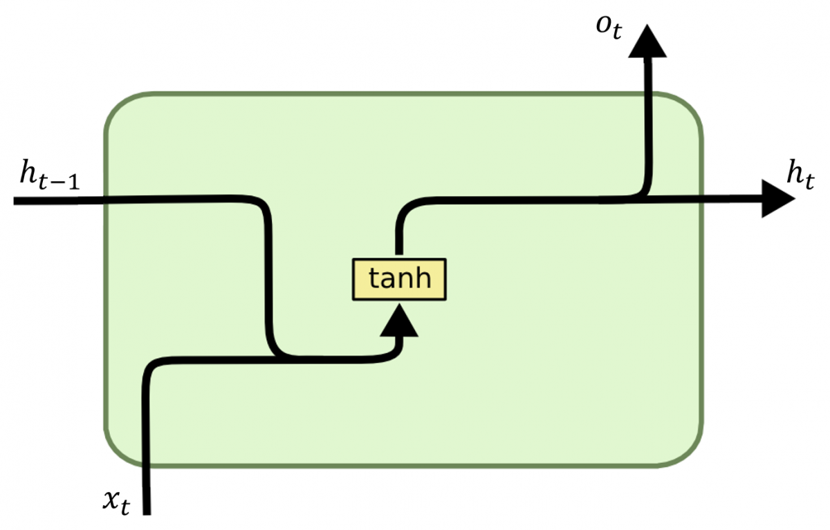
At each time step $t$, an RNN takes the current input $x_t$ and the previous hidden state $h_{t-1}$ to compute the new hidden state $h_t$:

$$
h_t = f(W_h h_{t-1} + W_x x_t + b_h)
$$

where:

• $W_h$ and $W_x$ are weight matrices,
• $b_h$ is the bias term,
• $f$ is usually a non-linear activation function like $ \tanh $,
• $h_t$ represents the memory of past computations.

Finally, the output $o_t$ is computed as:

$$
o_t = g(W_y h_t + b_y)
$$

where $g$ is often a softmax function for classification tasks.

The Vanishing Gradient Problem

A major challenge in training RNNs is the vanishing gradient problem.
During backpropagation, gradients can shrink exponentially when passing through many time steps, making it difficult to learn long-range dependencies.

To address this issue, LSTMs (Long Short-Term Memory) and GRUs (Gated Recurrent Units) were introduced.

Long Short-Term Memory (LSTM)

LSTMs introduce gates to control how much past information should be retained or discarded. This helps preserve long-term dependencies.

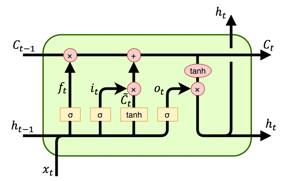
Each LSTM unit has:

1. Forget Gate: Decides what information to discard
   $$
   f_t = \sigma(W_f h_{t-1} + U_f x_t + b_f)
   $$
2. Input Gate: Determines new information to store
   $$
   i_t = \sigma(W_i h_{t-1} + U_i x_t + b_i)
   $$
3. Cell State Update: Computes the candidate memory

$$
\tilde{C_t} = \tanh(W_c h_{t-1} + U_c x_t + b_c)
$$

Then updates the cell state:

$$
C_t = f_t C_{t-1} + i_t \tilde{C}_t
$$

4. Output Gate: Determines the final hidden state
   $$
   o_t = \sigma(W_o h_{t-1} + U_o x_t + b_o)
   $$
   $$
   h_t = o_t \tanh(C_t)
   $$

LSTMs ensure that important past information remains accessible over long sequences.

Cell State $C_t$

The cell state can be considered as the “memory” of the LSTM network. It carries information across time steps, and it’s responsible for helping the network preserve long-term dependencies. The cell state is essentially the backbone of an LSTM that allows it to remember information over long sequences.

Update Mechanism of Cell State

The cell state is updated through two important gates in the LSTM:

1. Forget Gate ($f_t$) - Decides what information should be discarded.
2. Input Gate ($i_t$) - Determines what new information should be added to the memory.

The cell state $C_t$ is updated as follows:

$$
C_t = f_t \cdot C_{t-1} + i_t \cdot \tilde{C}_t
$$

Where:

• $C_{t-1}$ is the previous cell state.
• $f_t$ is the forget gate’s output, which decides how much of the previous cell state should be remembered.
• $i_t$ is the input gate’s output, which decides how much new information should be stored in the cell state.
• $\tilde{C}_t$ is the candidate cell state, which represents the new potential memory.

Hidden State $h_t$

The hidden state is the network’s short-term memory. It represents the output of the LSTM at each time step and carries information relevant to the current time step’s computation. The hidden state is the value that is passed to the next time step and is typically used to generate predictions or outputs.

Update Mechanism of Hidden State

The hidden state $h_t$ is derived from the current cell state $C_t$ using the output gate ($o_t$). The output gate decides how much of the current cell state should be exposed as the hidden state:

$$
h_t = o_t \cdot \tanh(C_t)
$$

Where:

• $o_t$ is the output gate, which determines how much of the cell state should be visible in the hidden state.
• $\tanh(C_t)$ is the cell state passed through the $\tanh$ activation function.

Differences Between $C_t$ and $h_t$

While both cell state ($C_t$) and hidden state ($h_t$) are crucial in LSTM networks, they serve distinct roles:

• $C_t$ (Cell State):

  • Acts as the long-term memory of the network.
  • It is designed to carry information over long time periods, ensuring the network remembers relevant data from earlier time steps.
  • The cell state is passed through the time steps with minimal changes unless explicitly modified by the forget and input gates.

• $h_t$ (Hidden State):

  • Acts as the short-term memory.
  • It contains information that is relevant to the current time step and is used to generate the output of the LSTM at each time step.
  • The hidden state is passed to the next time step as the updated memory, which is used for prediction or classification.

Gated Recurrent Unit (GRU)

GRUs are another variant of RNNs introduced to improve the learning of long-range dependencies. GRUs are simpler than LSTMs, as they use fewer gates, which can lead to faster training times while still addressing the vanishing gradient problem.

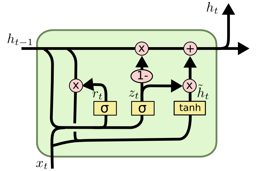
A GRU unit consists of two main gates:

1. Update Gate: This gate decides how much of the past information should be carried forward.
   $$
   z_t = \sigma(W_z h_{t-1} + U_z x_t + b_z)
   $$

   $z_t = 0$: The model keeps the previous hidden state $h_{t-1}$ and does not update with new information.
   $z_t = 1$: The model fully updates the hidden state with the new candidate hidden state $\tilde{h}_t$.

2. Reset Gate: This gate determines how much of the past hidden state should be forgotten.
   $$
   r_t = \sigma(W_r h_{t-1} + U_r x_t + b_r)
   $$

   $r_t = 0$: Forget the previous hidden state.
   $r_t = 1$: Use the previous hidden state fully.

The candidate hidden state $\tilde{h}_t$ is computed as:

$$
\tilde{h_t} = \tanh(W_h (r_t \cdot h_{t-1}) + U_h x_t + b_h)
$$

Finally, the hidden state $h_t$ is updated as a combination of the previous hidden state and the candidate hidden state:

$$
h_t = (1 - z_t) \cdot h_{t-1} + z_t \cdot \tilde{h}_t
$$

The update gate controls how much of the previous hidden state is kept, while the reset gate determines how much of the past information is discarded.

GRUs are computationally more efficient than LSTMs because they have fewer parameters to train, yet often perform comparably in many tasks.

LSTM vs. GRU: Key Differences

While both LSTMs and GRUs address the vanishing gradient problem, their architecture and gate structure differ:

1. Number of Gates:

   • LSTM has three gates: Forget gate, Input gate, and Output gate.
   • GRU has only two gates: Update gate and Reset gate.

2. Complexity:

   • LSTM is generally more complex and has more parameters due to the extra gates and the cell state.
   • GRU is simpler with fewer parameters, making it computationally more efficient.

3. Performance:

   • LSTM might perform better on some tasks due to its ability to separately maintain the cell state and hidden state, but it may require more data and computational resources.
   • GRU, being simpler, can often match or even outperform LSTM on smaller datasets or simpler tasks.

4. Use Cases:

   • LSTM is typically used when the task requires more complex learning of long-term dependencies.
   • GRU is useful for faster training and can be an effective choice for tasks where slightly fewer gates might still work well.

In many practical scenarios, both LSTM and GRU can give similar results. The choice between the two often comes down to the specific task, available computational resources, and performance requirements.

Applications of RNNs

RNNs and their variants (LSTM, GRU) are widely used in:

Natural Language Processing (NLP)

• Sentiment analysis
• Machine translation (Google Translate)
• Chatbots & conversational AI

Time Series Forecasting

• Stock price prediction
• Weather forecasting

Speech Recognition

• Voice assistants like Siri & Google Assistant

Music Generation

• AI-generated compositions