Transformer ( Part 2: Multi-Head Attention )

Before the Transformer, sequence models like RNNs and LSTMs suffered from long-term dependency issues and low parallelization efficiency. Self-Attention was introduced as an alternative, allowing for parallel computation and capturing long-range dependencies.

However, a single-head Self-Attention mechanism has a limitation:
It can only focus on one type of relationship or pattern in the data.

Multi-Head Attention overcomes this by using multiple attention heads that capture different aspects of the input, improving the model’s expressiveness.

Single-Head Self-Attention

Before diving into Multi-Head Attention, let’s first understand how a single-head Self-Attention works.

Query, Key, Value

In Self-Attention, each input vector is mapped into three vectors:

• Query (Q): Represents the feature to search for.
• Key (K): Represents candidate features.
• Value (V): Represents the actual information to be aggregated.

Each token in the input has a corresponding $(Q, K, V)$ triplet.

Computing Attention Scores

For a given Query $Q$ and Key $K$, we compute a similarity score using scaled dot-product attention:

$$
\text{Attention}(Q, K, V) = \text{softmax}\left(\frac{QK^T}{\sqrt{d_k}}\right) V
$$

where:

• $QK^T$ computes similarity between Query and Key.
• $\sqrt{d_k}$ scales down the values to prevent large gradients.
• softmax ensures that attention weights sum to 1.
• The weights are applied to the Value $V$.

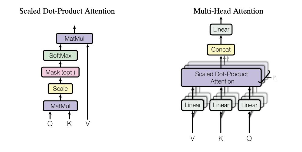
Multi-Head Attention Mechanism

A single-head Self-Attention mechanism only captures one perspective of the input relationships. Multi-Head Attention uses multiple heads to process different aspects of the sequence in parallel.

Computation Process of Multi-Head Attention

Multi-Head Attention follows these steps:

1. Linear Projections:

   • The input embedding $X$ has a dimension of $d_{\text{model}}$ (e.g., 512).

   • For each attention head, separate Query, Key, and Value vectors are computed using different linear transformations:

     $$
     Q_i = X W_i^Q, \quad K_i = X W_i^K, \quad V_i = X W_i^V
     $$

     where $W_i^Q, W_i^K, W_i^V \in \mathbb{R}^{d_{\text{model}} \times d_k}$ are learnable parameters.

2. Compute Attention for Each Head:
   Each attention head performs scaled dot-product attention:

   $$
   \text{head}_i = \text{Attention}(Q_i, K_i, V_i) = \text{softmax}\left(\frac{Q_i K_i^T}{\sqrt{d_k}}\right) V_i
   $$

3. Concatenation & Final Transformation:
   The outputs from all heads are concatenated and passed through a final linear transformation:

   $$
   \text{MultiHead}(Q, K, V) = \text{Concat}(\text{head}_1, …, \text{head}_h) W^O
   $$

   where $W^O \in \mathbb{R}^{h d_k \times d_{\text{model}}}$ is a trainable projection matrix.

Trainable Projection Matrix $W^O$

The final output of Multi-Head Attention is obtained by concatenating the outputs of all attention heads and applying a linear transformation using a projection matrix $W^O$. The matrix $W^O \in \mathbb{R}^{h d_k \times d_{\text{model}}}$ is a learnable parameter, meaning it is updated during training. Let’s break down what this means:

• $h$ represents the number of attention heads in the Multi-Head Attention mechanism. Each attention head processes the input in parallel, and having multiple heads allows the model to capture various relationships and features from the data.
• $d_k$ is the dimension of each attention head. Since the attention mechanism splits the model dimension ($d_{\text{model}}$) evenly across all heads, $d_k = \frac{d_{\text{model}}}{h}$.
• $\mathbb{R}$ refers to the set of real numbers. The notation $\mathbb{R}^{h d_k \times d_{\text{model}}}$ indicates that $W^O$ is a matrix with dimensions $h d_k$ by $d_{\text{model}}$, where the number of rows is the total dimension of all attention heads concatenated together, and the number of columns is the original model dimension.

Why is this Computation Necessary?

After the attention scores are computed and applied to the Values for each head, the outputs of all heads are concatenated. This concatenated output has a shape of $L \times h d_k$, where $L$ is the sequence length and $h d_k$ is the combined dimension of all attention heads. However, we want the final output of Multi-Head Attention to have the same dimension as the original input, $d_{\text{model}}$.

To achieve this, we use the projection matrix $W^O$, which transforms the concatenated vector back to the desired $d_{\text{model}}$ dimension. This ensures that the output from the Multi-Head Attention layer has the same dimension as the input, allowing it to be passed on to subsequent layers in the Transformer network without any dimension mismatch.

In short, the projection matrix $W^O$ enables the transformation of the concatenated attention head outputs into a final output with the same dimensionality as the input, ensuring consistency throughout the model.

Summary of Multi-Head Attention Formula

$$
\text{MultiHead}(Q, K, V) = \text{Concat}(\text{head}_1, …, \text{head}_h) W^O
$$

$$
\text{head}_i = \text{Attention}(QW_i^Q, KW_i^K, VW_i^V)
$$

where:

• $h$ is the number of attention heads.
• $d_k = d_{\text{model}} / h$ is the dimension of each head.
• $W^Q, W^K, W^V, W^O$ are learnable parameters.