About Machine Learning ( Part 10: Reinforcement Learning )

Introduction

Reinforcement Learning (RL) is a fascinating branch of machine learning where an agent learns to interact with an environment to maximize long-term cumulative rewards. Unlike supervised learning, RL relies on feedback through interaction instead of labeled data.

The core of RL is built upon Markov Decision Processes (MDPs), which provide a mathematical framework for modeling decision-making under uncertainty.

This blog post explores the key components of RL, including value functions, Q-functions, the Bellman equation, Actor-Critic architectures, PPO, and commonly used tools in real-world RL implementations.

What is Reinforcement Learning?

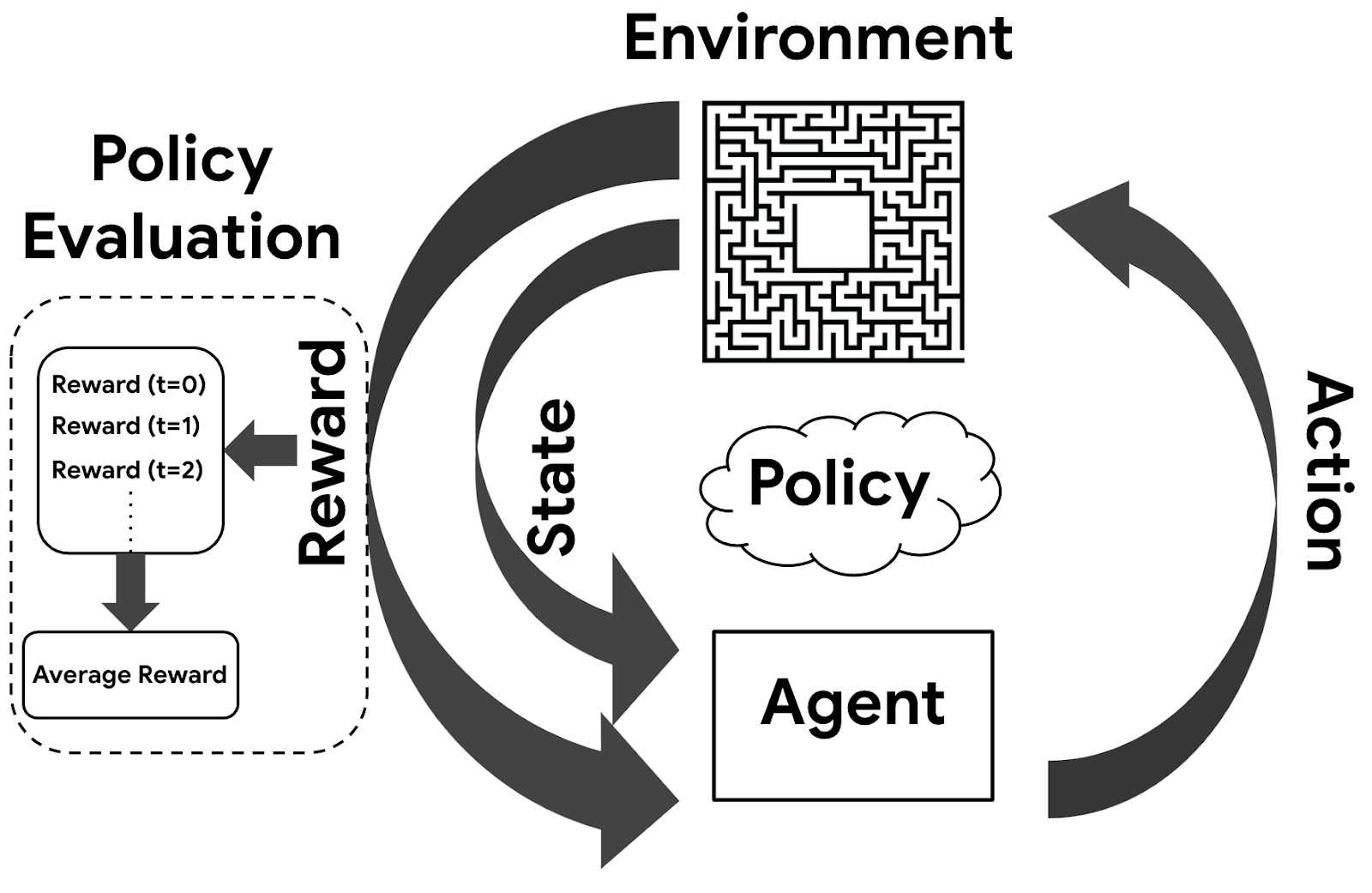
Reinforcement Learning involves an agent that:

• Observes a state $s$
• Takes an action $a$
• Receives a reward $r$
• Transitions to a new state $s’$
• Updates its policy $\pi$ to maximize long-term rewards

Key Concepts

Term	Description
Agent	The learner or decision-maker
Environment	The system the agent interacts with
State ($s$)	The current situation
Action ($a$)	A decision taken by the agent
Reward ($r$)	A scalar feedback signal from the environment
Policy ($\pi$)	A strategy mapping states to actions
Value Function ($V(s)$)	Expected return from state $s$
Q-Function ($Q(s,a)$)	Expected return from taking action $a$ in state $s$

Exploration vs. Exploitation

In RL, the agent must balance:

• Exploration: Trying unknown actions to learn about the environment
• Exploitation: Choosing the best-known action to maximize reward

This balance is crucial for learning an optimal policy without getting stuck in local optima.

Markov Decision Process (MDP)

An MDP formally defines an RL problem using:

1. States ($S$): Set of all possible states
2. Actions ($A$): Set of all possible actions
3. Transition Probability ($P(s’|s,a)$): Probability of transitioning to state $s’$ from state $s$ after action $a$
4. Reward Function ($R(s,a)$): Reward received when taking action $a$ in state $s$
5. Discount Factor ($\gamma$): A number in $[0, 1]$ that determines how much future rewards are worth

Markov Property

An MDP assumes the Markov property:

The future is independent of the past given the present.

This means the next state depends only on the current state and action, not on the sequence of events that preceded it.

Value Function and Q-Function

State Value Function $V(s)$

The expected return starting from state $s$ and following policy $\pi$ is:

$$
V(s) = \mathbb{E} \left[ \sum_{t=0}^{\infty} \gamma^t r_t \Big| s_0 = s \right]
$$

• $r_t$: reward at time step $t$
• $\gamma$: discount factor
• $\mathbb{E}_\pi$: expectation under policy $\pi$

Action-Value Function $Q(s, a)$

The expected return from state $s$, taking action $a$, and following policy $\pi$ is:

$$
Q(s, a) = \mathbb{E} \left[ \sum_{t=0}^{\infty} \gamma^t r_t \Big| s_0 = s, a_0 = a \right]
$$

• $a_0$: action taken at $t=0$

Bellman Equation

The Bellman Equation defines a recursive relationship for value functions.

For the value function:

$$
V(s) = \max_a \left( R(s, a) + \gamma \sum_{s’} P(s’|s, a) V(s’) \right)
$$

• $R(s,a)$: immediate reward
• $P(s’|s,a)$: transition probability
• $V(s’)$: value of the next state

For the Q-function:

$$
Q(s, a) = R(s, a) + \gamma \sum_{s’} P(s’|s, a) \max_{a’} Q(s’, a’)
$$

• $Q(s’, a’)$: estimated future return of next state and action

Actor-Critic Architecture

Actor-Critic methods use:

• Actor: Chooses actions based on policy $\pi$
• Critic: Evaluates the chosen action using $V(s)$ or $Q(s,a)$

This separation helps when:

• Rewards are sparse or delayed
• The environment is complex

The Critic provides guidance, helping the Actor improve its policy more efficiently.

PPO (Proximal Policy Optimization)

PPO is a modern Actor-Critic-based policy optimization algorithm that stabilizes learning through clipped surrogate objectives.

Workflow:

1. Interact with environment to collect experiences
2. Compute advantage estimates
3. Update Actor using a clipped objective
4. Update Critic by minimizing value loss
5. Repeat

PPO Objectives

1. Clipped Policy Objective:

$$
L^{CLIP}(\theta) = \mathbb{E}_t \left[ \min \left( r_t(\theta) \hat{A}_t, \text{clip}(r_t(\theta), 1 - \epsilon, 1 + \epsilon) \hat{A}_t \right) \right]
$$

• $r_t(\theta) = \frac{\pi_\theta(a_t|s_t)}{\pi_{\theta_{\text{old}}}(a_t|s_t)}$: policy ratio
• $\epsilon$: small hyperparameter controlling clip range
• $\hat{A}_t$: advantage estimate

2. Value Function Loss:

$$
L^{VF}(\theta) = \mathbb{E}_t \left[ \left( V_\theta(s_t) - \hat{R}_t \right)^2 \right]
$$

• $V_\theta(s_t)$: predicted value
• $\hat{R}_t$: actual return

3. Total Objective with Entropy Regularization:

$$
L(\theta) = L^{CLIP}(\theta) - c_1 L^{VF}(\theta) + c_2 S[\pi_\theta] (s_t)
$$

• $S\left[\pi_\theta\right] (s_t)$: policy entropy for encouraging exploration
• $c_1$, $c_2$: tuning coefficients

Why Use Advantage Instead of Raw Reward?

Using total return $\hat{R}_t$ directly to update the policy may be misleading due to:

1. State quality bias: Some states are inherently good/bad regardless of the action
2. High variance: Makes learning unstable

Instead, we compute the Advantage Function:

$$
\hat{A}_t = \hat{R}_t - V(s_t)
$$

• $\hat{R}_t$: estimated return from time $t$
• $V(s_t)$: critic’s estimate of state value

This tells us whether the action was better or worse than expected in a given state.

What is KL Divergence?

Kullback-Leibler (KL) Divergence measures how much one probability distribution diverges from another.

In PPO, it is used to:

• Monitor how much the new policy has changed from the old one
• Trigger early stopping or adjust learning rate if divergence is too high

GYM / Gymnasium

Gymnasium is a toolkit for building and testing RL environments.

Key Features:

• env.reset(): Initialize environment
• env.step(action): Apply action and receive next state, reward, done flag
• env.render(): Visualize environment
• observation_space, action_space: Define state/action formats

RL Tools & Components

Building effective reinforcement learning pipelines requires more than just algorithms — tooling is essential for stability, performance, and reproducibility. Here are some of the most important tools and components commonly used in practice:

Optuna is a powerful hyperparameter optimization library that automates tuning for better performance. It’s considered essential for finding optimal learning rates, network architectures, and other key parameters.

EvalCallback provides automated evaluation during training and saves the best-performing model. This helps avoid overfitting and ensures only the best version is deployed — an essential part of any RL workflow.

VecNormalize normalizes observations and rewards, which can significantly stabilize training, especially in environments with varying scales. It’s a crucial component for consistent performance.

CheckpointCallback periodically saves model checkpoints. This is highly recommended to prevent loss of progress and enable resuming long training sessions.

CustomCallback allows developers to inject custom logging, metric tracking, or interventions during training. It’s recommended when standard callbacks don’t meet specific needs.

SubprocVecEnv enables parallel environment execution, speeding up data collection by running multiple environment instances simultaneously. It’s particularly beneficial when using on-policy algorithms like PPO that require a lot of experience per update.

TensorBoard is a visualization toolkit that makes it easy to monitor metrics such as reward, loss, and learning rate over time. It’s widely recommended for debugging and presenting training progress.

saving and loading normalization statistics (like those from VecNormalize) is a must-have for consistency between training and inference. Without restoring these stats, the agent may perform poorly during evaluation or deployment due to mismatched input scales.