About Machine Learning ( Part 4: Decision Tree )

A Decision Tree is a supervised learning algorithm used for both classification and regression tasks. It organizes data into a tree-like structure, where each internal node represents a decision based on a feature, and each leaf node provides a prediction. Decision trees are simple, interpretable, and capable of handling both categorical and numerical data.

Classification Tree

A Classification Tree is a decision tree used for classifying data into distinct categories or classes. The main objective of a classification tree is to predict the category or class to which a given input belongs based on various features.

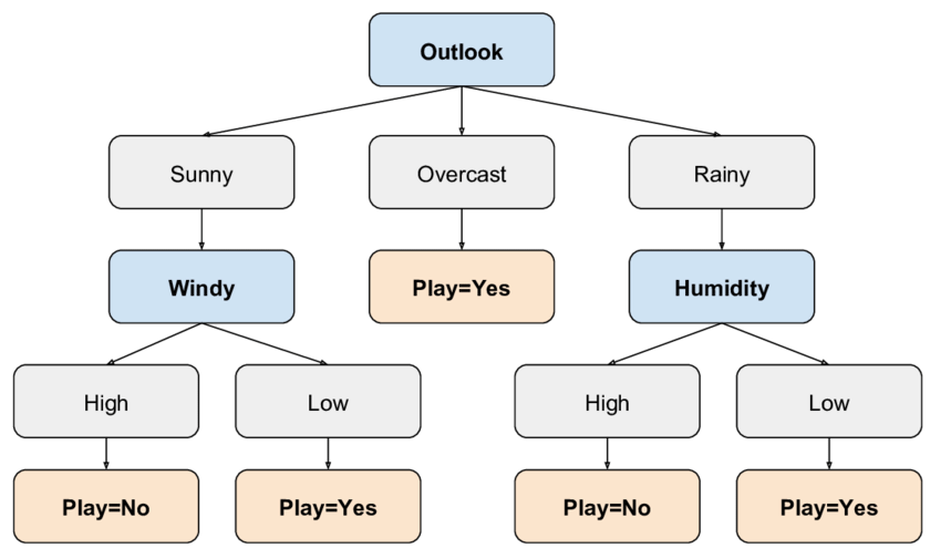
How Does a Classification Tree Work?

The tree is constructed in the following steps:

1. Select the best feature: The first step is to choose the feature that best splits the data. This is usually done by calculating the Entropy, such as Information Gain, or Gini Index.
2. Split the data: The chosen feature is used to split the dataset into two or more subsets. The splitting process continues recursively until the stopping criteria are met (e.g., maximum depth reached or all data in a node belong to the same class).
3. Predict the class: The leaf nodes represent the predicted class labels, which are determined based on the majority class in that node.

Entropy

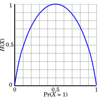
Entropy measures the disorder or uncertainty in a dataset. It quantifies the impurity of a dataset. If the dataset is perfectly pure (i.e., all samples belong to the same class), the entropy is 0. If the dataset has an equal distribution of all possible classes, the entropy reaches its maximum value.

The formula for entropy $H(S)$ of a set $S$ is:

$$
H(S) = - \sum_{x \in S} p(x) \log_2 p(x)
$$

Where:

• $S$ is the dataset.
• $p(x)$ is the proportion of instances in $S$ that belong to class $x$.

For binary classification (i.e., two classes, say “Yes” and “No”), the entropy simplifies to:

$$
H(S) = - p(+) \log_2 p(+) - p(-) \log_2 p(-)
$$

Where:

• $p(+)$ is the proportion of “Yes” labels in the dataset.
• $p(-)$ is the proportion of “No” labels in the dataset.

Interpretation of Entropy:

• If the entire dataset belongs to one class (e.g., all “Yes” or all “No”), then the entropy is 0 because there is no uncertainty.
• If the dataset has an equal distribution of both classes (e.g., $p(+) = p(-) = 0.5$), the entropy is 1 because there is maximum uncertainty.

For example, in the case of a Tennis Playing dataset, if the target variable (whether a person will play tennis or not) is evenly split between “Yes” and “No”, the entropy will be:

$$
H(S) = - 0.5 \log_2 0.5 - 0.5 \log_2 0.5 = 1
$$

This means the data is maximally uncertain (a 50/50 chance of playing or not playing).

Information Gain

Information Gain (IG) measures how well an attribute (or feature) separates the dataset into distinct classes. It is based on the difference in entropy before and after the split. The goal is to reduce uncertainty or disorder in the data as much as possible by selecting the attribute.

The formula for Information Gain when splitting a dataset $S$ based on an attribute $A$ is:

$$
IG(S, A) = H(S) - \sum_{v \in V(A)} \frac{|S_v|}{|S|} H(S_v)
$$

Where:

• $H(S)$ is the entropy of the dataset $S$ before the split.
• $H(S_v)$ is the entropy of the subset $S_v$.
• $V(A)$ is the set of all possible values for attribute $A$.
• $\frac{|S_v|}{|S|}$ is the proportion of the data in subset $S_v$ relative to the entire dataset $S$. ( Weighted )

The higher the information gain, the better the attribute is at reducing uncertainty and distinguishing between different classes. A high information gain indicates that the attribute is good at separating the data into pure subsets.

Code Demo

Gini Index

Gini Index is another measure used to evaluate the quality of a split in a decision tree. It measures the impurity or disorder of a dataset, with a lower Gini index indicating a purer dataset.

The Gini index for a dataset ( S ) is calculated as:

$$
Gini(S) = 1 - \sum_{i=1}^{C} p_i^2
$$

Where:

• ( C ) is the number of classes in the target variable.
• ( p_i ) is the proportion of the samples in the dataset ( S ) that belong to class ( i ).

Interpretation:

• If all the data points belong to a single class, the Gini index is 0, indicating a pure node.
• If the data points are evenly distributed among all classes, the Gini index is maximized (impure node). For binary classification, the maximum value is 0.5.

Overfitting

Overfitting occurs when a decision tree becomes too complex, capturing noise in the data instead of general patterns. It performs well on training data but poorly on new data.

Given a hypothesis space $H$, a hypothesis $h \in H$ is said to overfit the training data if there exists some alternative hypothesis $h’ \in H$, such that $h$ has a smaller error than $h’$ over the training examples, but $h’$ has a smaller error than $h$ over the entire distribution of instances.
– Tom Mitchell

Causes: Noisy data or insufficient data can lead to overfitting.

Solutions:

1. Stop growing the tree once it reaches a certain depth.
2. Prune the tree by removing branches with little importance.

Pruning

Pruning reduces tree complexity by removing unnecessary nodes.

Process:

1. Turn a node into a leaf with the most common value in that subset.
2. Test the accuracy of the pruned tree.
3. If accuracy improves, keep the change; if not, restore the node.

Data Splits:

• Training set for building the tree.
• Testing set for evaluating performance.
• Pruning set for pruning decisions.

Benefits:

• Simplifies the model.
• Reduces overfitting and improves generalization.
• Results in better test data performance.

Regression Tree

A Regression Tree is a type of decision tree used for predicting continuous target variables. Unlike classification trees that predict discrete labels, regression trees predict numerical values. Here’s how the process works:

1. Choosing Features and Split Values

   • The goal is to find the best feature and threshold to split the data. This is done by minimizing the variance or mean squared error (MSE) within each subset after the split.
   • For example, given a feature $X$ and target $Y$, we want to find a threshold $t$ to split the data into two subsets: $X \leq t$ and $X > t$. The split that minimizes the variance within each subset is chosen.

2. Splitting the Data

   • Once the best feature and threshold are identified, the data is split into two subsets based on this threshold.
   • This is a recursive process, where each subset is further split until a stopping condition (e.g., maximum depth or minimum sample size) is met.

3. Recursive Splitting

   • At each node, the algorithm continues splitting based on the feature that minimizes the variance.
   • For example, a tree might first split the data based on $X = 5$, then further split the subset $X > 5$ based on $X = 7$.

4. Leaf Nodes and Predictions

   • When the tree reaches the stopping condition, each leaf node represents a final prediction, which is the mean target value of the data points in that node.
   • For instance, if a leaf node contains values $Y = 10, 12, 14$, the prediction for that leaf would be the average $12$.

5. Prediction for New Data

   • For new data, the tree traverses from the root to a leaf node, where the predicted value is the mean of the target values in that leaf.

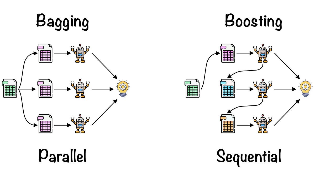
Bagging vs Boosting

In machine learning, Bagging and Boosting are two popular ensemble techniques used to improve the performance of models. These methods combine the predictions of multiple base learners to form a stronger model, but they approach this goal in different ways.

Bagging (Bootstrap Aggregating)

Bagging is an ensemble technique that reduces variance by training multiple base learners independently on different subsets of the data and then combining their predictions.

1. How Bagging Works

1. Data Sampling: Multiple subsets of the training data are created by random sampling with replacement (bootstrap sampling).
2. Train Multiple Models: Each subset is used to train a separate model, typically the same type of model (e.g., decision trees).
3. Combine Predictions: For classification problems, the final prediction is the class that receives the most votes from all base learners (majority voting). For regression problems, the final prediction is the average of all base learner predictions.

2. Advantages

• Reduces overfitting, particularly with high-variance models (e.g., decision trees).
• Works well with unstable base learners.

3. Disadvantages

• Doesn’t perform as well when base learners are weak or the model complexity is too high.

4. Example Algorithm

• Random Forest: A popular implementation of Bagging, where base learners are decision trees trained on random subsets of features.

Boosting

Boosting is an ensemble technique that improves weak learners by iteratively training them on the data and adjusting the weights to focus on the mistakes of previous models.

1. How Boosting Works

1. Train the First Model: Train a base learner on the training data.
2. Calculate Error: Calculate the errors made by the first model.
3. Adjust Weights: Increase the weights of the misclassified data points, so that the next model will focus more on them.
4. Train Subsequent Models: Train the next model using the updated weights.
5. Combine Predictions: The final prediction is a weighted average (regression) or a weighted vote (classification) of all base learners.

2. Advantages

• Reduces bias, improving model accuracy by focusing on hard-to-predict examples.
• Works well with weak learners that have high bias.

3. Disadvantages

• Can overfit if data is noisy or contains outliers.
• Computationally expensive since models are trained sequentially.

4. Example Algorithms

• AdaBoost: Adaptive Boosting is an ensemble learning method that combines multiple weak learners (usually decision trees) to create a strong learner. The goal is to improve predictive performance by focusing on the most difficult samples and iteratively adjusting the weights of misclassified samples.

  1. Initialization:
     AdaBoost begins by assigning equal weights to all training samples. If there are $N$ samples, each sample gets a weight of $\omega_i = \frac{1}{N}$.

  2. Train Weak Learner:
     A weak learner (a simple model, like a decision tree) is trained on the data. After each iteration, AdaBoost evaluates the classifier’s error rate.

  3. Error Rate and Classifier Weight:
     The error rate is calculated as the weighted sum of misclassified samples. The classifier’s weight ($\alpha$) is computed based on its error rate:

     $$ \alpha = \frac{1}{2} \ln\left( \frac{1 - \text{Error}}{\text{Error}} \right) $$

  4. Update Sample Weights:
     Based on the classifier’s performance, the weights of the training samples are updated:

     • For correctly classified samples, their weights are decreased.
     • For misclassified samples, their weights are increased.

     This makes the algorithm focus more on the samples that are hard to classify.

     The weight updates are:

     • Correct samples: $\omega_i \rightarrow \omega_i \times e^{-\alpha}$
     • Misclassified samples: $\omega_i \rightarrow \omega_i \times e^{\alpha}$
     • $\alpha$ is the weight assigned to the classifier based on its performance (error rate).

  5. Final Prediction:
     In the final prediction phase, the predictions of all weak learners are combined, with each learner’s prediction weighted according to its performance ($\alpha$). The final model is a weighted sum of all weak classifiers.

• Gradient Boosting: An improved version of Boosting that optimizes the model using gradient descent.

• XGBoost: A highly efficient implementation of Gradient Boosting, popular in machine learning competitions.