About Machine Learning ( Part 5: Support Vector Machine )

Support Vector Machine (SVM)

Support Vector Machines (SVM) are one of the most powerful supervised learning algorithms used for classification and regression tasks.

The Hyperplane

In a binary classification problem, the goal of SVM is to find a hyperplane that best separates two classes. Given a training dataset:

$$
D = { (\mathbf{x}_1, y_1), (\mathbf{x}_2, y_2), \dots, (\mathbf{x}_n, y_n) }, \quad \mathbf{x}_i \in \mathbb{R}^d, \quad y_i \in {-1, +1}
$$

• $\mathbf{x}_i$: $d$-dimensional feature vector (e.g., pixel values in an image).
• $y_i$: Class label ($+1$ for “cat”, $-1$ for “dog”).

The Hyperplane

A hyperplane in $\mathbb{R}^d$ is defined as:

$$
\mathbf{w} \cdot \mathbf{x} + b = 0, \quad \mathbf{x} \in \mathbb{R}^d
$$

• $\mathbf{w}$: Weight vector (normal to the hyperplane).
• $b$: Bias term (shifts the hyperplane away from the origin).
• $\mathbf{x}$: Any point in the feature space.

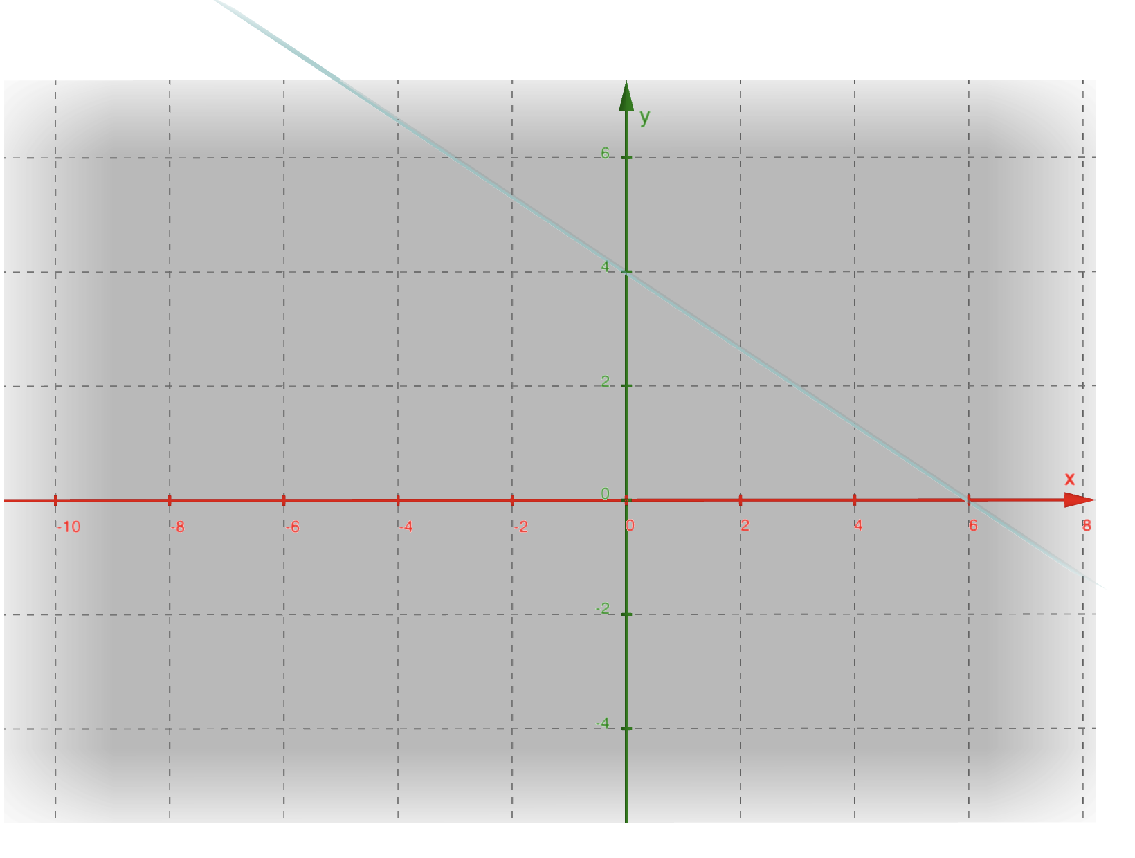
Example: 2D Hyperplane

Consider a 2D hyperplane $2x_1 + 3x_2 - 12 = 0$:

• Normal Vector: $\mathbf{w} = [2, 3]$.
• Bias: $b = -12$.

The weight vector $\mathbf{w}$ is perpendicular to the hyperplane.

Margin Maximization

The distance from a sample $\mathbf{x}_i$ to the hyperplane is:

$$
\text{Distance} = \frac{|\mathbf{w} \cdot \mathbf{x}_i + b|}{|\mathbf{w}|}.
$$

SVM seeks the hyperplane that maximizes the minimum margin between classes:

$$
\max_{\mathbf{w}, b} ( \frac{2}{|\mathbf{w}|} ) \quad \text{subject to} \quad y_i(\mathbf{w} \cdot \mathbf{x}_i + b) \geq 1, , \forall i.
$$

This is equivalent to minimizing $|\mathbf{w}|^2$, a convex optimization problem solvable via quadratic programming.

Optimize

Linear Separation with Hard Margin

When data is perfectly linearly separable, SVM seeks the hyperplane with maximum margin:

$$
\min_{\mathbf{w}, b} \frac{1}{2}|\mathbf{w}|^2 \quad \text{subject to} \quad y_i(\mathbf{w}^T\mathbf{x}_i + b) \geq 1, , \forall i
$$

Geometric Interpretation:
The margin width is $\frac{2}{|\mathbf{w}|}$. Maximizing margin = minimizing $|\mathbf{w}|$.

The Limitation:

Fails catastrophically when:

• Data has noise/outliers
• Classes are inherently non-separable

Soft Margin SVM

Allow controlled violations using slack variables $\xi_i$:

$$
\begin{aligned}
\min_{\mathbf{w}, b, \xi} &\quad \frac{1}{2}|\mathbf{w}|^2 + C\sum_{i=1}^n \xi_i \
\text{s.t.} &\quad y_i(\mathbf{w}^T\mathbf{x}_i + b) \geq 1 - \xi_i \
&\quad \xi_i \geq 0, \quad \forall i
\end{aligned}
$$

• $C$: Penalty weight (Large $C$ ≈ Hard Margin)
• $\xi_i$: How much the $i$-th sample violates the margin

Lagrangian Formulation

Convert constraints into the objective function:

$$ \mathcal{L} = \frac{1}{2}\|\mathbf{w}\|^2 + C\sum_{i=1}^n \xi_i - \sum_{i=1}^n \alpha_i[y_i(\mathbf{w}^T\mathbf{x}_i + b) - 1 + \xi_i] - \sum_{i=1}^n \mu_i\xi_i $$

Key Derivations:

1. Primal Variables

   • $\frac{\partial \mathcal{L}}{\partial \mathbf{w}} = 0 \Rightarrow \mathbf{w} = \sum \alpha_i y_i \mathbf{x}_i$
   • $\frac{\partial \mathcal{L}}{\partial b} = 0 \Rightarrow \sum \alpha_i y_i = 0$
   • $\frac{\partial \mathcal{L}}{\partial \xi_i} = 0 \Rightarrow \alpha_i + \mu_i = C$

2. Dual Problem
   Substitute back to get:

$$
\max_{\alpha} \sum_{i=1}^n \alpha_i - \frac{1}{2}\sum_{i,j} \alpha_i \alpha_j y_i y_j \mathbf{x}_i^T \mathbf{x}_j \
\text{s.t.} \quad 0 \leq \alpha_i \leq C, \quad \sum \alpha_i y_i = 0
$$

Interpretation of $\alpha_i$

$\alpha_i$ Range	Sample Status	$\xi_i$ Value
$=0$	Outside margin	0
$(0, C)$	On margin	0
$=C$	Inside margin	$>0$

Decision Function:

$$
f(\mathbf{x}) = \text{sign}( \sum_{\alpha_i > 0} \alpha_i y_i \mathbf{x}_i^T \mathbf{x} + b)
$$

Nonlinear Classification with Kernel Trick

The Fundamental Idea

Problem: Many datasets require nonlinear boundaries.
Solution: Map data to higher dimension $\phi(\mathbf{x})$ where linear separation becomes possible.

Example Transformation:
For $\mathbf{x} = [x_1, x_2]$, use $\phi(\mathbf{x}) = [x_1, x_2, x_1^2 + x_2^2]$

The Computational Challenge

Direct computation of $\phi(\mathbf{x}_i)^T \phi(\mathbf{x}_j)$ in high dimensions is intractable.

Key Insight: Many ML algorithms (like SVM) only need inner products, not explicit coordinates.

Kernel Functions to the Rescue

Replace $\phi(\mathbf{x}_i)^T \phi(\mathbf{x}_j)$ with kernel $K(\mathbf{x}_i, \mathbf{x}_j)$:

Updated Dual Problem:

$$
\max_{\alpha} \sum_{i=1}^n \alpha_i - \frac{1}{2}\sum_{i,j} \alpha_i \alpha_j y_i y_j K(\mathbf{x}_i, \mathbf{x}_j)
$$

Common Kernels:

Kernel	Formula	Characteristics
Linear	$K(\mathbf{x}, \mathbf{z}) = \mathbf{x}^T\mathbf{z}$	No transformation
Polynomial	$(\mathbf{x}^T\mathbf{z} + c)^d$	Captures polynomial interactions
RBF	$\exp(-\gamma |\mathbf{x}-\mathbf{z}|^2)$	Infinite-dimensional mapping
Sigmoid	$\tanh(\alpha \mathbf{x}^T\mathbf{z} + c)$	Mimics neural networks

3.4 Why Kernels Work: Mercer’s Theorem

A valid kernel must:

1. Be symmetric: $K(\mathbf{x}, \mathbf{z}) = K(\mathbf{z}, \mathbf{x})$
2. Produce positive semi-definite Gram matrix

Practical Check: If SVM training converges, your kernel is valid.